


 +26 rating, 28 votes
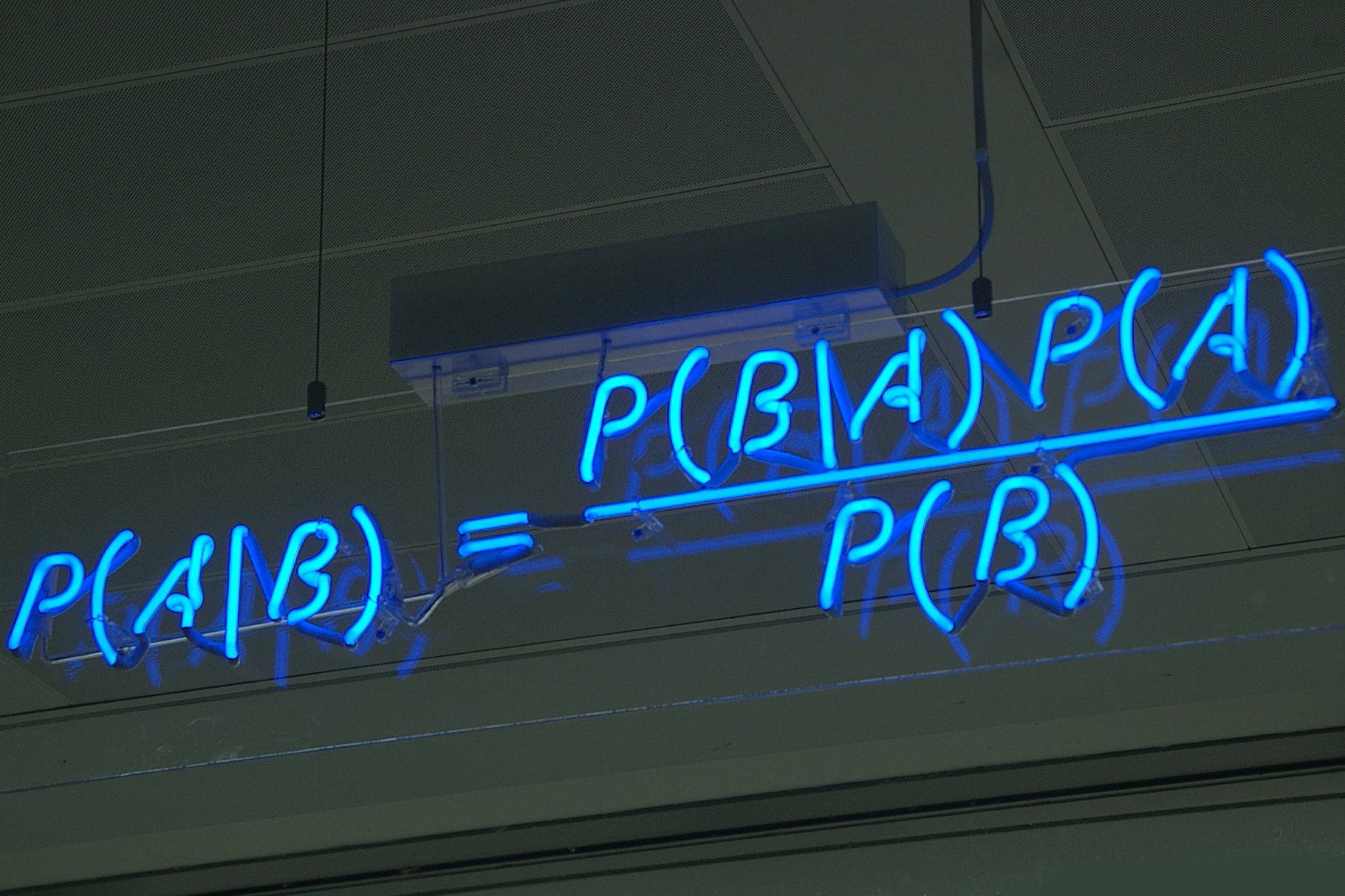

Introduction
Post last updated: 30.06.2015. Thanks to EP and others for pointing out that the negation signs were not always displayed properly in the formulae.
If some terrible catastrophe destroyed human civilization and humanity lost all scientific knowledge it ever collected – which single piece of information would you pass on to the survivors? Richard Feynman’s answer is the following:
All things are made of atoms – little particles that move around in perpetual motion, attracting each other when they are a little distance apart, but repelling upon being squeezed into one another.
Luke Muelhauser deems this an excellent choice, especially since it takes us a long way to reductionism. He suggests Bayes’ Theorem as the second piece of information he would choose. As he writes: “Seeing the world through the lens of Bayes’ Theorem is like seeing The Matrix. Nothing is the same after you have seen Bayes.”
Bayes’ Theorem tells us how to rationally assess the probability of a certain statement of interest being true, given some evidence. This could be the probability that a patient has a certain disease, the probability that a startup will be successful, or the probability that your opponent at the poker table has you beat. Insofar as science consists in creating hypotheses, collecting evidence for and against them, and updating our credence in these hypotheses in the face of the collected evidence, Bayes’ Theorem formalizes the very process of doing science.
As humans, we are all already more or less good at applying Bayes’ Theorem unconsciously. Imagine that while waiting in a train station, you notice a bag which has been left unattended for one hour. Could it be a bomb? “I guess people forget their bags on train stations much more often than they try to detonate bombs”, you reason. Cautiously, you move a bit closer to the bag and notice that there is something ticking inside the bag. What now? Are you getting nervous, or is a bomb still too unlikely? How should you rationally assess the probability that the bag actually contains a bomb? Which numbers would you need to know (and how many of them) in order to make a confident assessment? What would you actually do with these numbers?
It has been shown repeatedly that even well-trained people systematically deviate from correct Bayesian reasoning when confronted with examples such as the one given before. By definition, such a systematic deviation constitutes a cognitive bias. Consider the most well-known example:
Only 1% of women at age forty who participate in a routine mammography test have breast cancer. 80% of women who have breast cancer will get positive mammographies, but 9.6% of women who don’t have breast cancer will also get positive mammographies. A woman of this age had a positive mammography in a routine screening. What is the probability that she actually has breast cancer?
Can you find the correct answer? In case you can’t, make an estimate. Only 15% of all doctors are able to give the correct answer, and people who aren’t usually give answers above 70%, which is way too high. The correct answer is 7.8%. It is much easier to derive this result if the problem is phrased in terms of natural frequencies instead of percentages:
100 out of 10,000 women at age forty who participate in routine screening have breast cancer. 80 of every 100 women with breast cancer will get a positive mammography. 950 out of 9,900 women without breast cancer will also get a positive mammography. If 10,000 women in this age group undergo a routine screening, about what fraction of these women with positive mammographies will actually have breast cancer?
If the problem is phrased like this, more people are able to find the correct solution. It may also be more evident this way that we really need all three pieces of information to arrive at the solution: the fraction of women with breast cancer; the fraction of women with breast cancer who get a positive mammography; and the fraction of women without breast cancer who get a positive mammography.
People who give answers much higher than 7.8% usually neglect the first piece of information – the chance that a given woman has breast cancer if we don’t know the test result. For example, some people subtract 9.6% from 80%, which is completely wrong. It is important to realize that learning the test result does not simply replace our prior knowledge (in this example, that only 1% of women in the relevant demographic have breast cancer). It merely allows us to update our initial credence by a certain factor. Ignoring the prior probability and only relying on the evidence at hand is known in the psychological literature as base rate neglect.
A special case of base rate neglect is the prosecutor’s fallacy, with Sally Clark probably being the most prominent victim. As an example, suppose a robber was wearing a certain tattoo which only one person in 10,000 is wearing, and then a person wearing that tattoo is found. This does not imply that the chance of the suspect being innocent is 1 in 10,000, since the probability of any given person having been the robber is very small. Again, the correctly updated probability of the suspect being guilty needs to weight in both the prior probability of the suspect being guilty and the strength of the evidence provided by the tattoo.
The prior probability and the strength of the evidence correspond exactly to the two factors in Bayes’ Theorem. Before we can state it in a formal way, we need to introduce conditional probabilities.
Formal Matters
For an arbitrary event  (e.g., = “it will rain tomorrow”) we denote its probability by
  . Given two events and
  , we denote the probability of both of them happening by
  . Finally, we denote by
  the probability of given . For example, if = “there is a bomb in this bag” and = “there is something ticking in this bag”, then denotes the probability that there is a bomb in the bag if we’ve noticed that there’s something ticking inside. Conditional probabilities thus allow us to express how the probability of a hypothesis changes in the face of new evidence. In the above example, would denote the probability of a bomb in the bag before we noticed the ticking, and presumably we have
  .
.
The three quantities ,  , and are connected through the relation
(1) 
In words, the probability that and both happen is the probability that happens times the probability that happens, given that has happened. We can also condition on and write
(2) 
Combining these two equations, we find  . After dividing by and relabeling and to
  and
and  , respectively, we finally arrive at
(3) 
This is Bayes’ Theorem, which tells us how calculate the conditional probability  , where stands for hypothesis and stands for evidence. While from a formal point of view, Bayes’ Theorem follows trivially from the definition of conditional probabilities, it is an entirely different thing to internalize it and being able to correctly apply it in real-world problems.
The left-hand-side, tells us the probability of a hypothesis after updating this probability for the evidence . The first factor on the right-hand-side,  , is the prior probability, i.e., our credence in the hypothesis prior to the evidence . The denominator,
  is the probability of the evidence we are given, while
  is the probability of this evidence given our hypothesis.
In many practical examples, the denominator is not known directly but needs to be calculated first. In order to see how this can be done, we need one further bit of notation. For some event , we denote by  its negation. Correspondingly,
  denotes the probability that does not happen, and we have the evident relation
  (either happens or it doesn’t happen – there’s no third possibility). As a final requisite, we’ll need the relation
(4) 
If we apply this to the denominator p(E) in Bayes’ Theorem, we arrive at its most practically useful form
(5) 
Let us see how this applies to the breast cancer problem. In this case, denotes the hypothesis that the woman does have breast cancer and denotes a positive mammography. The prior probability of breast cancer is given by  , and consequently
  . If a woman does have breast cancer, the probability of a positive mammography is
  , while if she doesn’t have cancer, it is
  . Inserting all of these quantities in the above form of Bayes’ Theorem, we arrive at
(6) 
Can you apply Bayes’ Theorem to the following problem?
Suppose that a barrel contains many small plastic eggs. Some eggs are painted red and some are painted blue. 40% of the eggs in the bin contain pearls, and 60% contain nothing. 30% of eggs containing pearls are painted blue, and 10% of eggs containing nothing are painted blue. What is the probability that a blue egg contains a pearl? [1]
Besides giving a precise, formal meaning to commonsensical wisdoms such as “never be absolutely certain” or “update your credences when you see new evidence”, there are some less trivial lessons to be learned from Bayes’ Theorem. People often introduce a dichotomy between proofs and evidence that can be ignored. However, this distinction is a useful heuristic at best. Ultimately, all our beliefs should be probabilistic and ideally take into account all available evidence, be it weak or strong. An example is the saying “correlation does not imply causation”. Actually, observing an unexpected correlation between variables and does increase the probability that one of them causally influences the other, even if alternatives – such as a third variable  causally influencing both and or the data having been manipulated – may have considerable weight, too.
Similarly, the fact that people believed in Zeus’ existence is evidence that Zeus actually exists. If Zeus did exist, this would make it likelier that there are people who believe in him; therefore, people believing in Zeus is evidence for his existence. This statement can in fact be formally derived. The equation
(7) 
can be rearranged to
(8) 
Therefore,  if and only if
  . In words, evidence increases the probability of hypothesis if and only if hypothesis makes evidence more likely than we would otherwise expect. The prior probability of Zeus’ existence should be so low, however, that even after updating for the fact that myths about Zeus exist, the probability of his existence is still negligible for all practical purposes. (Why should this prior be so low? This will be discussed shortly.)
Similarly, and despite a more well-known aphorism stating the contrary, absence of evidence is evidence of absence. It follows from
(9) 
and  that
that
(10) ![\begin{equation*} 0 = \left[p(H|E) - p(H)\right] \cdot p(E) + \left[p(H|\neg E) - p(H)\right] \cdot p(\neg E) \end{equation*}](http://crucialconsiderations.org/wp-content/ql-cache/quicklatex.com-5212eca118d549bc2aa16ff65219e68e_l3.png "Rendered by QuickLaTeX.com")
So if and only if  ; if some evidence would increase our credence in hypothesis , then not observing evidence has to decrease our credence in . The fact that centuries of science have not collected any evidence that would allow us to increase our credence in Zeus’ existence should further decrease our credence in his existence.
More generally, any expected increase ![[p(H|E) - p(H)] \cdot p(E)](http://crucialconsiderations.org/wp-content/ql-cache/quicklatex.com-8c03c624518494f13d4acafbf164fec5_l3.png "Rendered by QuickLaTeX.com") in our credence for some hypothesis needs to be counterbalanced by an equally-sized expected decrease
in our credence for some hypothesis needs to be counterbalanced by an equally-sized expected decrease ![[p(H|\neg E) - p(H)] \cdot p(\neg E)](http://crucialconsiderations.org/wp-content/ql-cache/quicklatex.com-6a8a1259e355097346bc3b9941ee30f4_l3.png "Rendered by QuickLaTeX.com") . We cannot rationally have an expectation value for our future credence that differs from our present credence. If we expected to upshift a hypothesis stronger than we downshift it, this should already affect our current credence.
. We cannot rationally have an expectation value for our future credence that differs from our present credence. If we expected to upshift a hypothesis stronger than we downshift it, this should already affect our current credence.
Moreover, since  , one of the two summands and
  being small implies the other one being large (i.e., close to 1), and vice versa. Therefore, if we expect a high probability of weak evidence into one direction, this needs to be balanced by a low probability for strong evidence in the other direction. Eliezer Yudkowsky calls this principle the Conservation of Expected Evidence. The breast cancer case discussed in the introduction is an excellent example: We expect with high probability a negative result, which leads to a weak decrease of our credence in the woman having cancer (it was already as low as 1%); this is balanced by the rare event of a positive result, which is strong evidence for the woman having cancer.
Science and Priors
As stated in the introduction, Bayes’ Theorem formalizes the very act of doing science. For example, it gives a precise explanation for many ideas developed by Karl Popper, which are collectively known as falsificationism. At the core of falsificationism is the idea that theories can be definitely falsified, but never definitely confirmed. No matter how many white swans you observe, you can never definitely confirm that “all swans are white”; by contrast, observing a single black swan falsifies it. Formally, this directly follows from Bayes’ Theorem. If your theory  definitely forbids a certain observation
  –
–  – then observing definitely disconfirms your theory –
  . By contrast, given a finite set of observations it is impossible to update the credence in theory to
  if our prior probability (the probability we had before conditioning on evidence) was
  . Bayes’ Theorem tells us that we only could have if
  , i.e., if there were no theory other than that could predict . This is indeed something that we can never know – we can’t possibly exclude all theories other than . Newtonian mechanics was incredibly well-confirmed and nevertheless it turned out that it describes only a certain limit of Einstein’s more general theory of relativity.
Recall the Conservation of Expected Evidence rule, which states that an expected increase in the credence of a theory needs to be balanced by an equally sized expected decrease. This explains why it is so crucial that a theory be falsifiable. If it is impossible to decrease the credence in a theory, it is also mathematically impossible to increase it – and vice versa, which is where Popper was wrong. It is possible to probabilistically confirm a theory and thereby increase its likelihood. Confirmation and falsification are not fundamentally different, as Popper argued, but both just special cases of Bayes’ Theorem.
Finally, let us turn to the question of where priors, the value of the prior probabilities, come from, and how we should rationally choose them. Firstly, let us note that the choice of priors is not that important if we are given a sufficiently large set of data. The more updates of our probabilities we perform, the more they become independent of the priors. In practice, what prior to choose is often self-evident if the case we are interested in can be viewed as a random element of a larger group about whose statistics we have some information. For example, in the breast cancer case we can view the woman as picked at random from all the women in her demographic, and can then use the (known) fraction of women with breast cancer in that demographic as the prior probability of her having cancer. If we have more information on the woman, e.g. that she is 43 years old, we can use the cancer rate among 43-year-old women as a more precise prior, should we have this information available.
Even if we have no previous information, symmetries sometimes suggest a reasonable prior. Imagine having six bowling balls in front of you that are indistinguishable by eye. It is then natural to assign each ball a prior of 1/6 of being the heaviest, since there is simply no reason for assigning a higher probability to one ball than to another.
However, in many real-world problems, there is no obvious choice for coming up with a prior probability. What is the prior probability of Zeus existing, or of the universe being finite in size? In the 1960s, Ray Solomonoff developed what is known as the universal prior. The universal prior combines and formalizes ideas of philosophers Epicurus (341–270 BC) and William of Ockham (1287 – 1347). Epicurus’ principle states that one should keep all hypotheses that are consistent with the data. Ockham’s principle, widely known as Occam’s Razor, states that entities should not be multiplied beyond necessity. This is widely understood to mean: Among all hypotheses consistent with the observations, choose the simplest.
Solomonoff’s universal prior unifies these two principles. It gives all hypotheses consistent with the data a non-zero probability, but highest probability to the simplest ones. The technicalities necessary for a precise definition of how “simplest” is to be understood here are well beyond this text. However, we should stress that “simple” does not mean “easy to understand for a human”. Rather, complexity should roughly be thought of as the length of a computer program that is able to reproduce your hypothesis. The universal prior is exponentially small in this length and thus strongly penalizes hypotheses which involve unnecessary complications.
As an example, the explanation that Thor’s wrath is responsible for thunderstorms may sound simple enough to humans, and definitely simpler than atmospheric physics. However, a computer program that simulated Thor throwing lightning bolts needed not only to simulate the lightning bolts themselves, but Thor as well. Viewed from this perspective, Thor appears as an unnecessary complication, which does not in fact have any explanatory power. By contrast, the Standard Model of particle physics explains much, much more than thunderstorms, and its rules could be written down in a few pages of programming code.
We close with a historical example which shows that the choice of priors can sometimes be decisive if observations do not allow to exclude one of two rivaling theories. Both the (geocentric) Ptolemaic and the (heliocentric) Copernican model of the cosmos were able to explain all observations that Copernicus’ contemporaries could make. This means that the ratio of the credences in the two theories could not be changed through observations; it was determined by the priors alone. A prior that punishes ad hoc adjustments (which “increase the length of the program”), such as the proverbial epicycles in the Ptolemaic system, would lead to a strong preference for the Copernican model. Preferring a heliocentric model was thus the rational thing to do for Copernicus, even though he was not able to refute the geocentric model on empirical grounds.
Footnotes
1. The answer is 2/3.↩
References
Parts of this posting is based on Luke Muelhauser’s An Intuitive Explanation of Eliezer Yudkowsky’s Intuitive Explanation of Bayes’ Theorem
13.5%?
> Can you apply Bayes’ Theorem to the following problem?
I guess I’ll never know …
2/3 ?
I also got 2/3. I guess now that we have more believers in 2/3, it should be the more probable right answer? 😉
Well, I got 2/3 as A did.
What I did whas this:
p(P|B) = p(P) . p(B|P) / ( p(P) . p(B|P) + p(-P) . p(B|-P) )
p(P|B) = 0.4 x 0.3 / ( (0.4 x 0.3) + (0.6 x 0.1) )
p(P|B) = 0.12 / (0.12 + 0.06) = 0.12 / 0.18
p(P|B) = 0.6666666666666667 =~ 2/3
Is the answer 2/3?
I don’t understand the equation that sites between (9) and (10). It seems like the last P( E) term is missing a negation operator. Where does that equation come from?
the equation 9′ is indeed missing a negation in the last term. I think it comes from the law of total probability as E and not E are disjoint events upon which H depends.
Thanks for pointing this out EP! It was a problem with the latex conversion, it’s now fixed.
You’re welcome